Utility – Parts Per Billion

Risk and Rationality in Uncertainty

We have many philosophical ideas about how money is not everything in life but deep down, everyone knows how money constitutes to a bigger portion of who we are. Although money can’t buy everything, the unexplainable value it holds behind presence of almost everything in our lives will never go unnoticed. We know that this importance of money/ resources/ assets is highly dependent on how much of those we have right now and how much of those may get lost in an uncertain event. This perception of value drives our decision making in risky situations. The Expected Utility Theory (EUT) in economics deals with the modelling of such scenarios. The mathematical formalization of the perception of wealth and our risk profile is facilitated by this fundamental theory. EUT lies at the foundation of actuarial science/ insurance, financial risk management, decision making under budget restrictions, asset management, and investment management.

EXPECTED UTILITY THEORY

We live in an uncertain world. Timing events where too many interactions are happening could be risky especially when it comes to money or the basic resources for sustenance. In crisis situations, our survival instincts have always kicked in to ensure preservation of life and the resources required to ensure its longevity. They need not to be always rational, they are just meant to save life somehow, that is why most of the acts of survival seem extraordinary. Interesting thing to understand here is that when such extraordinary survival instincts kick in as a mass effect the whole mass effect becomes irrational, unexplainable, incoherent. There is no sane explanation to justify these mass events. When such events badly affect the resources responsible for basic life of every being, it can be catastrophic. Huge sudden falls in stock market are good indicators of such disasters, crises. Insurance on the other hand could prepare person to handle the disasters in a preventive way. Stock market and insurance are one of the best examples to understand how people assess risk and maintain/ reject rationality while making important decisions. We will see what formal ideas from economics lie behind these events of uncertainty.

Expected Utility Theory (EUT) in Economics

Expected utility theory lays the foundation of how a rational person would make decision in an uncertainty where valuable resources like money are involved. The whole idea is based on the quantification of that uncertainty and connecting that uncertainty with the individual gains from individual uncertain event. Expected utility also creates a formal structure of how person perceives risk in given scenario. This helps to quantify the value generated from any economic event.

Origin – St. Petersburg Paradox

Daniel Bernoulli is credited to establish the expected utility theory which is one of the foundations of economics. The theory emerged from the St. Petersburg Paradox which goes like this:

You have $2 and we toss a coin. Heads, the amount you have now is doubled and tails then the game stops and you leave with whatever amount you have right now. The game continues till its always heads in series and stops when the coin shows tails.

The question is how much will you be willing to pay to enter this bet?

The probability of heads and tails is 50-50% which is ½ . If it is a series of heads (heads followed by heads) then the events are dependent on each other, so the probability of this event is intertwined with the probability of the previous one. If there happens a game where you start with $2 and every time heads comes, and the money goes on doubling the equation of gain would be:

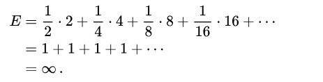
As this math goes, a person should pay infinite amount as he will be gaining infinite amount from such game. ‘E’ value here is identified as expected value. Even if one such possible game would happen in reality, people won’t pay infinite amount in reality to enter this bet.

Bernoulli resolved this paradox by creating the concept of Expected utility. People will pay not what actual value it delivers (as in the $s of money); they will pay according to how actually it will be useful to them, ‘utilizable’ to them – that is where the utility and thus expected utility comes in picture.

Expected utility is calculated by the amount one would gain and the chances of gaining that amount. The expected utility thus is sum of all the gains connected with the probabilities of gaining them.

Daniel Bernoulli
The determination of the value of an item must not be based on its price, but rather on the utility it yields.

1^st Tenet of EUT: Expectation

The overall utility of a prospect, is the expected utility of its outcomes.

In very simple words, for a given scenario you will weigh the chances of its constituent events and connect them with their respective gains. The sum of the all connections of each gain with their chance of realization is the usefulness – utility of that scenario.

Mathematically,

Expectation:

In our example we need to assume something that is the usability of the money – utility.

We assume $10 has utility of 1 unit. (This is just an assumption to understand the concept. When multiple objects are involved, their utilities will be different.)

So, the expected utility of this scenario is:

E = ((1000/10)x0.2) + ((50/10)x0.65) + (10000)x0.15) =

20 + 3.25 + 150 = 173.25 units

So, the expected utility – the usefulness of this event is 173.25 units.

The unit of value which we assumed in this calculation is sometimes called ‘utils’ – the basic unit of utility. It will change based on how one perceives the value in given scenario.

You will realize that the expected utility is the weighted average of utility of events and their individual probabilities.

Four Axioms of Utility Theory

Later John von Neumann and Oskar Morgenstern expanded the concept of EUT with the idea of rationality. The agents involved in such uncertain economic exchanges are ‘econs’-the rational beings.

They have clear preferences among the options provided in every economic decision which comes under the idea of “completeness”. If out of the given set they select multiple options at a time, then it is said that they are ‘indifferent’ to these options. Whatever might be the internal distribution of constituent they might have. It’s about the final utility they perceive. When presented with choices, a rational person has clear preferences for those choices.

For all given uncertain events there is a hierarchy of preferences. If A is preferred over B and B is preferred over C, then A is always preferred over C. Which goes as transitivity.

Suppose we have been presented three events where event A is preferred over B and B is preferred over C. Now if one introduces a new event N which is slightly less preferred than B and more preferred over C then event B and N would be indifferent. In simple words, the choices between options would never directly jump, they will align as per the preferences in line.

So, A>B>C and B>N>C then A>B>C and A>N>C mean the same.

This is continuity. Graphically, the utility function is always a smooth curve.

Why do A>B>C and A>N>C mean the same even when the calculated numeric value would differ? It is because utility is never an absolute value it is just used to arrange the preferences by quantifying them. Ground rules used to define usability from the given resources i.e., the utility function of given scenario will be different for different scenarios and different sets of people. This is simplification of the concept called ordinality of utility. You can rank utility but not say that event A is this many percent better than event B.

When you have set the preferences of A over B and if you are offered another totally different/ irrelevant event M with new utility. You would still prefer A over B. Introduction of M will not affect the preferences as if A and B are independent of M. This is called ‘independence‘ in EUT.

So, completeness, transitivity, continuity and independence are the four axioms of EUT. Note that they are not ‘complete’ representation of reality. It’s just that they bring in simplicity to treat given scenarios and evaluate them. That is why you will find contradictions to these axioms. (Maybe a topic for another time.) The axioms are there to create a formal mathematical structure to draw useful inferences.

2^nd Tenet of Expected Utility Theory: Asset Integration

In EUT, asset integration is an idea based on the assumption that all people making economic decisions are rational. So, in uncertainty or risky scenarios a rational person will look at the overall gains instead of focusing on one certain gain and neglecting other unsure gains. A rational person will look at the risks of scenarios in a collective way and decide to enter only if the expected utility improves his assets’ position. A rational person will only enter the given scenario if the collective utility is better than the individual utility of its sub-events or sub-gains.

A rational person will not focus on an individual more probable gain even when his overall gains are becoming low.

3^rd Tenet of Expected Utility Theory: Risk

The beautiful insight EUT creates is about the mathematical formalization of risk profile. For that we will understand some ideas in advance.

Utility function – it is a mathematical relation between how one sees the value of given object/ resource. The value of resources is different for different people. A crude example would be how a beggar values money for one time meal compared to a filthy rich person. The value of $25 would be different for different people based on the conditions they are in.

This is where marginal utility comes in picture.

Marginal utility talks about what difference it makes in your perception of the value of a given thing if one would give you more of that in the next event. Roughly speaking the more we have something, the less we value it, so marginal utility is always diminishing. If I already have 10 packets of chocolates which are enough for the day to me, the next 11^th packet of chocolate won’t make that much difference in my current excitement of having 10 packets. (Please note that we are talking about rationality here, although nobody is rational when it comes to chocolates.) A rational version of me would trade that 11^th packet for something else with a person who hasn’t received even a single packet. A person who has no chocolate would perceive that single packet with higher value than how I perceived it (provided that he loves chocolates).

Alfred Marshall – the British Economist brought the concept of
‘Marginal Utility’ through his book ‘Principles of Economics’ in 1890.

So, utility function is a mathematical transformation of objects in given event to a unitary value so that the results can be easily compared with each other because the transformation converts everything to single unit system. These single unit of value is called ‘util’.

Utility function can be any possible mathematical relation. Generally, it is expected to be simple to not invite the complexities in modeling of given economic scenario. It should be simple enough to draw realistic conclusions.

An understanding of utility function gives insight into how the person evaluates risk with respect to the resources they hold.

Consider a scenario:

Event 1 – You enter a lottery where there is 50% chance that you will win $100 and 50% chance that you win nothing.

Event 2 – You are given $50 for sure, unconditionally just for playing the lottery.

Assume we have three differently thinking people to make choices in this scenario. Different thinking means how they assess the risk of entering the lottery which has some uncertainty and the surety of winning $50. Difference in assessment of risk means difference in the perception of utility. It further means that the utility function will be characteristic to each person.

Person 1 has the following utility function:

So, for Person 1 the utility of certainty (7.07 utils) is higher than the uncertainty (5 utils). He is happy to walk away with sure $50 gain instead of betting for $100 lottery.

Person 1 doesn’t want to take risk by entering the Event 1 of betting when he is sure about gain of $50 in Event 2. This is risk-averse behavior. The utility function mathematically models that risk averse behavior. Utility function is concave in risk aversion.

Now comes Person 2 with the following utility function:

You will see that the utility of certain and uncertain choices is the same. It means that it doesn’t matter for this guy if he enters the lottery having uncertainty or gets $50 for sure. This is risk-neutral behavior. The person 2 doesn’t care about certainty or uncertainty. He values both events the same. As mathematically both have similar utilities. Person 2 is indifferent to both events.

Now see the Person 3 with following utility function:

This guy has a radical view, he perceives the worth of entering the lottery (5000 utils) better than gaining $50 for sure (2500 utils). This guy is gambler! He finds it more interesting to enter the bet instead of gaining $50 for sure. He is happy to take the risk in uncertainty.

Looking at these three people you should note that the scenarios/ events they are presented are exactly the same. The only thing which is different is how they see the value in lottery and the sure gain.

So, the first person demonstrates risk averse behavior. He wants surety of gain rather than gambling for higher but unsure gain.

The second person demonstrates risk neutral behavior. Bet or no bet he doesn’t care. Just be done with it.

The third person demonstrates risk loving behavior. He wants the thrill of uncertainty in betting, so he sees more value in uncertainty of lottery.

This is how Expected Utility Theory can be implemented to mathematically model how different sets of people/fund managers will make decisions based on the risk profile. The relation between expected utility (which is the weighted average of gains) and utility function (which shows how one values the gain) can show us the risk profile.

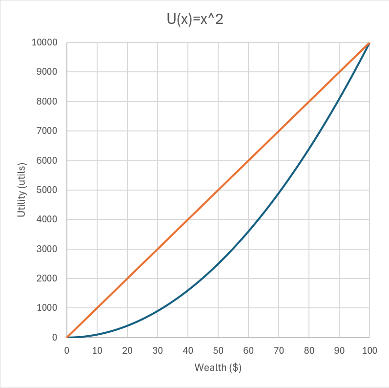
In the graphs shown, blue lines show utility function and the orange lines show expected utility. The orange line in our case connects the utility of $100 and $0 which is Event 1. This orange line connects any points on utility curve and it will give the expected utility value for that scenario of uncertain gain. In simple words, it’s the line of weighted average exactly like the definition of expected utility. This line is used to find out the certainty equivalent (CE). A certainty equivalent is the utility of an uncertain gain if it was certain.

Almost all the time, people are risk averse. People want to avoid uncertainty about higher gains when they are presented with some lower but sure gain. This is where marginal utility becomes important. (This point deserves broad explanation which we will cover another time under Prospect Theory)

Marginal Utility

In risk averse people, you will see that the utility function starts to flatten out once the value gained increases. The more value someone already has the less he values the next addition of bunch into the preexisting bulk. Remember the chocolate box example?

One with 10 boxes of chocolate perceives one additional box with less value, whereas some with no chocolate will see it as a precious one as he has nothing right now. The perceived value of the additional next lot goes on reducing. This is known as diminishing marginal utility. Marginal utility is always diminishing.

So, a safe playing person would stop entering the next gamble because he now has enough. The next uncertainty in gambling has less value for him.

EUT in actuarial

Now it is obvious that only a risk averse person would go for conservative approach in uncertainty. This also means that risk aversion will also invite preventive measure against loss of certain assets, resources. Insurance thus comes into the picture. EUT here helps to mathematically formalize the probability of the risks which would compromise current gains, the perceived value of asset/ property/ resource and losses one can bear. We can now calculate the premium for the insurance against uncertainty of loss of something.

So, we will look into a scenario where risk aversion exists thus marginal utility is always diminishing.

We have the utility function of a man has a property giving revenue of $100K/year as:

u(x)=ln x

Now will see the risk scenario. Suppose this person does a fire audit of his property and the auditing agency finds out that there is 50% chance that he will suffer a loss of $60K/year due to fire hazard and 50% chance that nothing will happen.

After rephrasing, the gains from the property would look this:

50% chance that the income is $40K/year and 50% chance that income is $100K/ year.

Using the tenets of EUT the mathematical expression becomes:

Now, what we are doing differently here is to find out what this expected utility in uncertainty means when there is complete effect of loss with some chance and gain of some chance. In earlier examples we had second event of certainty against which we compared to understand the risk profile. Now it’s reverse calculation, we know the risk profile, we know the perceived overall value i.e., EUT of the property. Now we will find the certainty equivalent (CE) using the risk profile which can be explained by the utility function of the person.

How much is this 11.05 utils in terms of money from the property for this guy? We can find this from utility function of the person.

ln(x)=11.05, thus x=$63245.55

Now, think the fire hazard as a lottery where you gain $63245.55 money as per EUT calculation. Whether the fire will happen or not, the possible overall earning from this property would be $63245.55.

Now, if the property without any fire hazard was giving me $100k and the insurer guarantees me that same earning for the losses due to hazard. How much maximum amount should I pay to the insurance agency?

I will pay only that much amount which falls short to the $100k when compared to perceived earning calculated from the combined effect of certainty and uncertainty as given by EUT.

My earing due to uncertainty is $63.2k/year, I would receive $100 for a fine year so in order to continue that $100k even for a worse year I would pay insurance agency = $100000 – $63245 = $36754.45.

Anything I am paying above $36754.45/ year for insurance premium is loss for me. I would not go above this amount to insure my property which guarantees income of $100k per year. This is how the insurance premium is decided.

Conclusion:

We have many philosophical ideas about how money is not everything in life but deep down everyone knows that money constitutes a bigger portion of who we are. Although money can’t buy everything, the unexplainable value it holds behind presence of almost everything in our lives will never go unnoticed. We know that this importance of money/ resources/ assets is highly dependent on how much of these we have right now and how much of those may get lost. This perception of value drives our decision making in risky situations. The mathematical formalization of the perception of wealth, our risk profile is facilitated by expected utility theory. Although this theory has its own limitations it lies at the foundation of the economics.

For further reading:

Von Neumann, John, and Oskar Morgenstern. “Theory of games and economic behavior: 60th anniversary commemorative edition.” Theory of games and economic behavior. Princeton university press, 2007
Kahneman, Daniel., and Amos Tversky. “Prospect theory: An analysis of decision under risk.” Econometrica 47.2 (1979): 363-391
Thinking fast and slow – Daniel Kahneman
Connecting money with sentiments – Behavioral Economics
Settling accounts with the losses – On Prospect Theory

The Utility of Human Life and Morality

Why doesn’t Batman kill all his villains once for all? Why the sentence passed by judicial systems in certain heinous and extraordinary crimes feel unjust for the pain victim went through? How one can tell that given person was right or wrong when he/she had no intent of doing it? Can you just look at the end consequences of the actions and decide right or wrong for such scenes? Jeremy Bentham’s philosophy of Utilitarianism tried to answer some of these questions but it revealed certain flaws in our ways of judgement. Even though hedonism and utilitarian philosophy create an objective model of morality, they fail to address the subjective and human aspect of any moral discussion. It reveals that the purpose of living is not mere happiness but self-improvement thereby mutual and overall improvement.

How to judge morality and its impact on human life?

The Moral Dilemma

A healthy sense of good and bad makes a society livable. There are some special, rare events that happen in the society we live which challenge our idea of what is good and what is bad. There are uncountable offenses and also in varying types which create problem of who should actually be punished and what should be the punishment.

An eye for an eye will make the whole world blind.
Mahatma Gandhi

If this is really the case, the law and order should punish the victim in such a way that it prohibits the future perpetrators to not do such crimes again. But again, as this above mentioned quote goes if the punishment given for the crime is equally dangerous then what exactly are we trying to establish through such punishment?

It’s like that scenario where murdering a murderer creates a new murderer so the net number of murderers in the society remain the same. An Italian philosopher called Cesare Bonesana di Beccaria had given a thought on this. In his book ‘Of Crimes and Punishments’ he discusses that if the punishments grow on crueler and crueler the net mindset of people also grows crueler. It’s like how water levels itself irrespective of the depths. The baseline of what is right and wrong furthermore what is more wrong and what is more right shifts up. Crueler and crueler crimes reduce the sensibility of people of that society. This could be one reason why people always argue that the judicial system does not provide equivalent punishment as a justice to the victims of certain heinous, exceptional cases of crimes. (Although there are many other factors to make such decisions.)

“In proportion as punishments become crueler, the minds of men, as a fluid rises to the same height with that which surrounds it, grow hardened and insensible; and the force of the passions still continuing, in the space of a hundred years the wheel terrifies no more than formerly the prison. That a punishment may produce the effect required, it is sufficient that the evil it occasions should exceed the good expected from the crime, including in the calculation the certainty of the punishment, and the privation of the expected advantage. All severity beyond this is superfluous, and therefore tyrannical.”
Cesare Beccaria, Of the Mildness of Punishments from ‘Of Crimes and Punishments’

In similar spirit, the relationship between Batman and Joker can be understood. Joker never cares about killing people he will try to stretch the limits of batman in every possible sense where innocent lives are at stake. Batman has one solution to stop all this – to kill the Joker. But with a high moral ground Batman would never kill Joker. What is the motivation behind such character design of Batman. Batman knows that killing Joker would solve the problem once for all. Believe me, this is not just a fictional comic book scenario. The reality that we live in has uncountable such scenarios where exactly same decision dilemmas occur.

The famous trolley problem also points to somewhat similar moral dilemma. Where should the trolley be directed if one track has single person and another has 5 people tied to the track? Nobody wants blood on their hands.

But the same trolley problem becomes interesting if you start adding additional attributes to the people who are on track.

What if the single person tied to the track is a scientist with the cure for cancer and the track with five people are criminals? Then definitely you would kill the five criminals instead of the single scientist.

Did you notice what change made us to decide faster? The moment we understood the consequences of our actions we had the clarity of what is right and what is wrong. Our moral compass pointed to North the moment we foresaw the consequences of our actions.

The foundation of some of the principles of morality are based on similar ideas. Utilitarianism and Jeremy Bentham’s an English Philosophers ideas have contributed to the ideas of morality for humanity, especially when we are talking about the human society as a whole. The ideas put by Jeremy Bentham also faced severe criticism, we will see those in detail too. But the key intention of my exploration is to understand how we create the meaning of Morality and how subjectivity, objectivity totally change the way we perceive morality. In the end we may reach to rock bottom questioning the morality itself to be nonexistent – and if morality is non-existent then what separates human beings from animals? (I hope to enter in this territory with some optimism, I don’t know where will it end.)

Utilitarianism

As I already explained in the trolley problem that by adding one simple, short part of information shifted our moral compass in (supposedly) proper direction. What did this information add in the dilemma to make it solvable?

The answer is the foresight of consequence. Once you saw the consequence it leads to you got the hold of what is right and what is wrong. You decided one side to be right and other one to be wrong. This foresight of consequence helped you to weigh the ‘right’-ness of your decision.

Utilitarianism is based on the measurement of morals based on the consequences of the actions you take. What is the other side of taking actions? It is ‘the intent’. This is where the fun game begins.

Many philosophers are always fighting over morals based on the intent of the person and the consequences of the actions they take. For example, thinking of murder (pardon my thinking) makes me less of convict than really murdering someone. My thinking has not led to the loss of the person I hate. Utilitarianism thus calls out for the construct of morality based on the actual actions and their consequences; it’s like saying ‘what a man is more about what he does instead of what he thinks’.

Hedonism, Utilitarianism and Jeremy Bentham

Happiness is a very pretty thing to feel, but very dry to talk about.
Jeremy Bentham

Jeremy Bentham an English philosopher contributed to the utilitarian ideas of morality. He was not well appreciated in his home country due to the misalignment of his ideas of socio-political reforms with the British sovereignty of those times. The French translation of his works on law, governance gave him popularity in Frenchmen. Bentham was one of the people who pushed the political reforms during French revolution.

While reading Joseph Priestly’s Essay on the First Principles of Government, Bentham came across the idea of “greatest happiness for the greatest number” which motivated him to expand the ideas of utilitarianism.

Priestly brought the idea of “Laissez-faire” (‘allow to do’ in French)- a policy of minimum governmental interference in the economic affairs of individuals and society. Joseph Priestly developed his ideas of politics, economics and government based on the ideas created by Adam Smith (Author of the Wealth of Nations – the holy grail of classical Economics).

The Greek philosopher called Epicurus was the supporter, creator of hedonism. Hedonism defines ethics to pleasure or pain. According to hedonism that which gives pleasure is morally good and that which give pain is morally wrong. The idea behind hedonism is the aversion of pain to live an undisturbed life because anyways this all won’t make sense once you are dead. According to Epicurus – fear of death, retribution is pushing people to collect more wealth, more power thereby causing more painful life. The collection of wealth, power is done thinking that they can avert the death but that is not the reality. So, worrying about the death sucks out the pleasure of living the life which itself is equivalent of death.

Non fui, fui, non-sum, non-curo
(“I was not; I was; I am not; I do not care”)
Epicurus

So, epicurean hedonistic morality tries to maximize the pleasure. The other end of this idea is that if everyone tries to maximize their own pleasure (egoistic hedonism) wouldn’t it disturb others?

If I want to listen to a song on loud speaker while bothering my neighbors, what is the moral standpoint here?

The answer is the overall good of the system. So, if you neighbor also wants to listen music loud and overall loud music is good for the group then we are morally right to play loud music. (Just pray that the group has same music interests!)

So, Jeremy Bentham is known to rejuvenate this ancient philosophy of egoistic hedonism through his philosophy of utilitarianism.

The basic idea behind Utilitarianism is to maximize the utility of anything, value of anything. The utility can be increased by doing what is right which can be done by doing what gives more pleasure or by avoiding those things which increase or give pain.

Utility is a property which tends

To produce benefit, advantage, pleasure, good or happiness
To prevent happening of mischief, pain, evil or happiness

So, the right action is the one that produces and/ or maximizes overall happiness. Please understand that the word “overall” is important for Jeremy Bentham’s philosophy of Utilitarianism. Because from selfish point of views, what is pleasurable for one may not be pleasurable for others. (This is also where the certain philosophical problems of Utilitarianism are hiding, save this point for later.)

To solve this bottleneck of clarity, there are two types of pleasure in human life – one is happiness from senses, physical experiences and one is from intellect. The intellectual happiness is higher than the pleasure from senses. So, on personal moral dilemmas these two attributes can solve the problem.

All good on personal level but what about the moral decisions for the group, for society? Here, Bentham solved the moral dilemma by using the idea of “greater good for all”. When we don’t agree on what makes us happy together, making sacrifices in your happiness to make others happy is the solution. (Keep this idea parked in your mind.)

“Nature has placed mankind under the governance of two sovereign masters – pain and pleasure. They govern us in all we do, all we say and all we think.”
Jeremy Bentham

Felicific Calculus – Measuring happiness

Jeremy Bentham is known as the Issac Newton of the Morality for developing the felicific calculus/ hedonistic calculus. Bentham pointed out the key factors which affect the net happiness and using this factors’ effect as a whole, one can quantify the happiness.

Following are the factors which affect the happiness:

Intensity – how strong is the pleasure from the given action?
Duration – how long does the happiness remain from given action?
Certainty – what is the likelihood of given pleasure to occur?
Propinquity – how soon/ immediate is the occurrence of the pleasure?
Fecundity – what is the possibility that this pleasure will also lead to the newer pleasure(s)?
Purity – what is the change that this pleasure will not bring some opposite sensation?
Extent – how many people are affected?

If one considers these factors and the principle to maximize the communal happiness, most of the social moral dilemmas can be effectively solved.

So, according to this felicific calculus,

Batman should kill the Joker for the greater good of the Gotham
The trolley should go over the group/ person which creates more pain for the society
Baby Hitler should be killed once we get the chance to travel back in time

You must appreciate the clarity which the felicific calculus brings. This clarity is very important for the policymakers, politicians while deciding the fate of the group, state, nation as a whole.

Now a simple question –

If batman keeps on killing the villains, won’t he become the greatest killer of them all? What would differentiate Batman from other villains?

What would happen if you were given false information about the nature of the people tied on track while riding that trolley? Could your wrong decision be undone? If it was the wrong decision then now ‘you’ are morally wrong, with the blood of the innocents.

You would kill baby Hitler only because you have vision that this baby will grow up to be the mass murderer tyrant. The mass murder hasn’t happened yet. So, now you are the killer of a ‘now’ innocent baby.

Maintaining same emotion, now you would appreciate why even for a strong judicial system giving capital punishment for rapists, terrorists is difficult morally. You would solve the problem for now because the act has been already done, the consequences have already happened (which is why moral judgement is effective as it relies on the consequences). Killing the perpetrators or punishing them with equal pain would definitely bring peace of mind using the principles of morality but that also degrades the morality of innocents who fell down from that morality. It is not matter of what one deserves because what bad happened to them, it is about how less human you will become once you perform that act of punishment.

Recall the quote of Beccaria in the early part of my discussion.

Killing joker will create fear among other villains but it also creates chance for the creation of even dangerous villain in future.

Killing baby Hitler doesn’t guarantee prevention of World War and mass murders, as our personalities are the result of our surroundings – another Hitler-like person would have emerged in such given circumstances. (I honestly don’t know if he/she would be worse or less harsh than the original one but you get the point – conditions anyways would have created another cruel person.)

Jumping out of the trolley seems the best way to run away from the pain of murder of other unknown people (joking). The trolley dilemma remains dilemma.

Also, the felicific calculus allows pain for small groups for the betterment/ pleasure of the bigger society. For example, according to this utilitarian idea killing few healthy convicted prisoners to save lives of many innocent people by harvesting the prisoners’ organ is justified. It is for the good in the end.

You see where this goes?

See the level to which any human or a group could go if they start justifying their moral rightness using these ideas. Using these principles any big group can overpower the minorities in morally right way. It is just a matter of time that the felicific calculus principles would get exploited for other “immoral” gains.

That is exactly why many people criticized the felicific calculus saying that a pig laying in the mud for his whole life would be happiest than a human being (Socrates to be specific) if Bentham’s calculus is used to decide morality.

In a crude way, there are two type of Utilitarianism which help to solve the problem to certain extent, but it is not a complete solution:

Act Utilitarianism – to act for the greater good of all
Rule Utilitarianism – to set rules in such way that no one inherently gets the pain or everyone is happy because actions and their consequences are bound by certain set rules in first place now

Happiness is not the ‘only’ and the ultimate goal – the limitations of Jeremy Bentham’s Utilitarian Philosophy

What people were not ‘happy’ with Jeremy Bentham’s felicific calculus was that it made humans more like machines and very objective. People don’t always want happiness for their or the group’s greater good. Exercising daily, reducing fat-sugar maybe painful but that guarantees healthy, illness free long life. Doing drugs isolates the person from pain but it impacts the long-term physical and mental health of the person. Hardships and pain make people to reach their difficult goals which is what is the real and ultimate happiness for them.

Happiness is not always the goal of life, if one is completely tangled in the pleasures of life and if everyone is having same mentality then in the end no one will be happy, because as a group we all would never agree on what makes us happy; different environments in which we grew, our personal experiences, our upbringing, our motivations prevent us from creating a common definition of happiness.

The subjective factor of pleasure or pain is not present in Bentham’s philosophy of Utilitarianism. Building further upon that, the victim who has suffered from the morally wrong action will only be satisfied when he/she gets justice, not when they are made happier than their perpetrators. (This justice must again not be mechanical and objective like the felicific calculus.)

One more flaw of the Bentham’s utilitarianism is the imbalance between personal scenarios and the communal scenarios. In most cases, it demands personal sacrifice irrespective of their subjective morality for the betterment of the group. (that is exactly how many past cruel dictators have justified their moral correctness on their acts against the minorities.)

A British philosopher, Bernard Williams presented a thought experiment to highlight such flaw of the Utilitarianism.

In this thought experiment:

A botanist on his South American expedition is ordered by the cruel regime soldiers to kill one of the Indian tribe people. If the botanist fails to kill one Indian the soldiers would execute all of the tribe members.

So, if we implement utilitarian principles, then the botanist should kill one Indian to save the remaining all. That is morally right.

But on the other hand, one must also understand that the botanist has nothing to do with the cruel regime and even with the indigenous tribe members. He is under no moral obligation to do anything. The consequences are in such a way that whatever he will do he will be called morally wrong. Which in the end is wrong.

The utilitarian philosophy neglects this subjectivity and consequentialism while we are deciding morality of anything.

Maybe that is also why even when we have all the rules in place, penal code in place for all types of offenses, similar crimes – we have a judge – a subjective, consequential observer to grant the final justice.

You must understand that the discussion does not want to pose Utilitarianism as completely wrong idea. The intent of this discussion is to understand how to de-clutter a complex moral scenario and how to inject subjectivity in it so that the correct person will get the justice in the end. As we are human beings and not machines, every day brings new subjective scenarios with new subjective moral dilemmas. Direct implementation of utilitarianism may bring in the transparency in the moral puzzle but it is at the expense of oversimplification and loss of personal subjectivity, consequential personal point of view and also freedom of person to exist.

The ways in which Utilitarianism brings immediate clarity by elimination of some important subjective aspects is dangerous and limits the judgement of real morality. Friedrich Nietzsche had warned new philosophers in his book beyond good and evil about the philosophies which create such “immediate certainties” like Utilitarian philosophy creates-

“The belief in “immediate certainties” is a moral naivete which does honor to us philosophers; but – we have now to cease being “merely moral” men!”
Friedrich Nietzsche

Conclusion – If not happiness then what is the goal of being human?

Jeremy Bentham’s philosophy of Utilitarianism and the felicific calculus can help to decide the morality of what is good for all but it ignores the presence and worth of personal integrity, the well being of the minorities, subjectivity of the person in given consequences. It by default eliminates the possibility of humans remaining human beings instead it attributes them as the machine maximizing a targeted outcome (which is pleasure here).

So, the question remains – If we are not meant to maximize pleasure during our tenure in life because in the end after death there will not be anything to experience or gain happiness – if our existence and final purpose does not align with being happy then what exactly is the purpose of being a human being?

Based on my understanding on what many great people have commented about the purpose of life, I found that most of them point to remaining the human being you always were. I am not saying that the personality should remain the same, rather it should change and keep on upgrading itself till the end but the core should remain same or it should not degrade at least.

Some wrong events, injustice, oppression, cruelty will make you suffer, but that should also not vilify your human spirit. Once we let go the pursuit of happiness and chase the goal of being a better human being (or at least remain the human being you are) we can fulfill the purpose of our lives and also make other people’s lives better.

Once you will let go of such utilitarian, mechanistic setups of morality you will realize that people don’t need gods, religions, governments, judicial systems to keep in the check of right and wrong. Our inner compass is more than enough to take care of what makes us human beings, this inner compass is not about what is right and wrong, for me it is about what better version of yourself you would become if you act in that certain way. It takes care of what you are thinking and what would be the consequences of actions thereby resolving the dilemma of morality which got separated on the basis of either intent or the consequences.

I am highlighting the importance of inner personal human compass because the rules designed to keep morality in check would always need revision and the utilitarian philosophy would wait for the consequences to happen to decide the morality. The goal of human struggle to improve their current version to a better one does not need either of the metrics to decide the morality.

Imagine what the world would become if everyone started appreciating this inner human compass!

(For now, we can only imagine, but I am optimistic on this.)

P.S. –

Even though the Utilitarian philosophy had many flaws, Jeremy Bentham contributed largely to bring in new political reforms, improve governance, establish penal codes in judicial systems, define sovereignty, reduce the influence of religious institutions on the lives of people and governments. His works were strategically maligned by some lobbies to lessen the impact of his other notable works. He was the proponent of liberty and freedom from religious influences on lives of people. The pushed for the establishment of a secular educational institute in London – now famously known as University College London. Jeremy Betham’s fully clothed wax statue containing his original skeleton remains in the entrance hall of the University main building upon his request.